Idle> /control/execute week01.mac
A Monte Carlo primer, before the first line of Geant4.蒙特卡罗入门:在写第一行 Geant4 之前。
You build a small Monte Carlo in pure Python: sample muon directions, send them through a two-layer telescope, count what arrives, and attach an uncertainty to the count. Every later Geant4 measurement in this course pays the same statistical tax you meet here.
先用纯 Python 写一个小型蒙特卡罗:抽样缪子方向,让它们穿过双层望远镜,统计到达的数目,并给结果配上不确定度。本课程之后每一个 Geant4 测量都要缴纳你在这里第一次遇到的“统计税”。
Overview概览3 min3 分钟
/run/initializelearning goals学习目标
By the end of this week you can put an error bar on a simulation.本周结束时,你能给模拟结果配上误差棒。
- State the Monte Carlo method蒙特卡罗方法 as repeated random sampling whose spread gives the uncertainty.把蒙特卡罗方法Monte Carlo method表述为重复随机抽样,并由样本的涨落给出不确定度。
- Sample isotropic directions correctly (cosθ uniform) and keep the beam model separate from the geometry.正确抽样各向同性方向(cosθ 均匀),并把束流模型与几何分开。
- Estimate a conditional transmission probability条件透射概率 ε = k/N with σε = √(ε(1−ε)/N), and tell it apart from acceptance and efficiency.用 ε = k/N 和 σε = √(ε(1−ε)/N) 估计条件透射概率conditional transmission probability,并把它与接受度、效率区分开。
- Show the 1/√N scaling of the statistical uncertainty统计不确定度 and use it to plan how many events a measurement needs.演示统计不确定度statistical uncertainty的 1/√N 标度,并据此估算一次测量需要多少事例。
- Check a Monte Carlo result against an independent expectation and quote the difference in units of σ.把蒙特卡罗结果与独立的预期值比较,并以 σ 为单位给出差异。
Reading阅读9 min9 分钟
/control/echo backgroundbackground · for non-physicists背景知识 · 写给非物理专业
A Monte Carlo is a way to get an answer by rolling dice many times.蒙特卡罗方法:用“掷很多次骰子”得到答案。
Background · Monte Carlo in engineering terms工程语言里的蒙特卡罗
If you have estimated a failure probability by sampling random loads and strengths, you have already done Monte Carlo. Here the random inputs are a muon's direction and entry point, the model is a straight line, and the output is a yes/no: did it cross both detector layers? The fraction of yes answers estimates the probability.
如果你曾通过随机抽取荷载和强度来估计结构的失效概率,你就已经做过蒙特卡罗了。这里的随机输入是缪子的方向和入射点,模型是一条直线,输出是“是/否”:它穿过两层探测器了吗?回答“是”的比例就是概率的估计值。
Background · Why the error shrinks only as 1/√N为什么误差只按 1/√N 缩小
Each trial is a coin flip with probability ε. Counting k successes in N trials has a spread of √(Nε(1−ε)), so the estimate k/N has an uncertainty of √(ε(1−ε)/N). Ten times more trials buy only √10 ≈ 3.2 times more precision. Real muon counting obeys the same rule, which is why muography surveys take days.
每次试验都像一次概率为 ε 的抛硬币。N 次试验中成功 k 次,其涨落为 √(Nε(1−ε)),所以估计值 k/N 的不确定度是 √(ε(1−ε)/N)。试验次数增加十倍,精度只提高 √10 ≈ 3.2 倍。真实的缪子计数遵循同样的规律,这就是缪子成像勘测要持续好几天的原因。
Background · cos²θ: why most muons come from overheadcos²θ:为什么大多数缪子来自头顶
θ is the zenith angle, measured from straight down. Muons arriving at a slant cross much more air, so fewer survive and they are more energetic. Near 3 GeV the result is an intensity roughly proportional to cos²θ: at 60° it is a quarter of the vertical value.
θ 是天顶角,从竖直向下方向量起。斜着来的缪子要穿过多得多的空气,存活下来的更少,能量也更高。在 3 GeV 附近,强度大致正比于 cos²θ:60° 时只有竖直方向的四分之一。
For muography projects用于缪子成像工程
The quantity you compute this week, ε, is a conditional transmission: of the muons that cross the upper layer, how many also cross the lower one. It is one ingredient of a telescope's geometric acceptance AΩ (m²·sr), which also needs the layer area and the solid angle. In a muography survey, AΩ × sky intensity × time gives the number of muons expected along each line of sight, the first number in any feasibility study for a tunnel or slope. Section 1.2 below explains the difference.
本周计算的 ε 是条件透射概率:穿过上层的缪子中,有多少也穿过下层。它只是望远镜几何接受度 AΩ(m²·sr)的一个组成部分,AΩ 还需要探测层面积和立体角。在缪子成像勘测中,AΩ × 天空强度 × 时间,给出每条视线上预期的缪子数,这是隧道或边坡可行性研究中要算的第一个数。下面 1.2 节说明二者的区别。
New to muons, units such as g/cm² or m.w.e., or muography? Start with the background primer.还不熟悉缪子、g/cm² 或米水当量这类单位,或缪子成像?先读入门背景。
Event display事例显示3 min3 分钟
/vis/open TSGevent display事例显示
Your Monte Carlo, drawn ray by ray.把你的蒙特卡罗一条一条画出来。
Reading阅读9 min9 分钟
/control/manual1.1 · why Python first1.1 · 为什么先用 Python
Ten new ideas on one screen is a problem of order, not of difficulty.一屏十个新概念,问题在于顺序,而不在于难度。
Open an official Geant4 example and you meet, on one screen, C++ syntax, the CMake build, detector construction, physics lists, the primary generator, user actions, sensitive detectors, visualization macros and random-number management. None of these is hard alone. The order is wrong, because no experimental question tells you why each class is needed.
打开一个官方 Geant4 示例,同一屏上会出现 C++ 语法、CMake 构建、探测器构建、物理列表、初级粒子产生器、用户动作、灵敏探测器、可视化宏和随机数管理。单独看每一项都不难,难的是顺序不对:没有一个实验问题告诉你为什么需要某个类。
This course reverses the order. You first finish a Monte Carlo experiment in Python, then move the same experiment into Geant4. When you meet G4ParticleGun next week you already know what "firing a particle" means. Only the language changes.
本课程把顺序倒过来:先用 Python 完成一个蒙特卡罗实验,再把同一个实验搬进 Geant4。下周遇到 G4ParticleGun 时,你已经知道“发射一个粒子”是什么意思,变的只是语言。
Example 1.1 · Today's laboratory question今天的实验问题
A plastic scintillator on your bench is read out by a PMT and an oscilloscope. Cosmic-ray muons cross it at random. Before building any Geant4 geometry, answer a simpler question: if muons arrive randomly, what fraction of sampled trajectories transmit through the telescope, and how much statistical uncertainty should you expect after a given number of events?
实验台上一块塑料闪烁体接 PMT 和示波器,宇宙线缪子随机地穿过它。在搭建任何 Geant4 几何之前,先回答一个更简单的问题:如果缪子随机到达,抽样径迹中有多大比例能穿过望远镜?给定事例数后,应当预期多大的统计不确定度?
Definition 1.1 · Monte Carlo method蒙特卡罗方法
The Monte Carlo method is a class of numerical techniques that solve deterministic or stochastic problems through repeated random sampling随机抽样. You build a probabilistic model for the quantity sought, draw and tally samples repeatedly, estimate the true value from the sample statistic, and take the uncertainty from the statistical fluctuation.
蒙特卡罗方法是一类通过重复随机抽样random sampling来求解确定性或随机性问题的数值方法:为所求的量建立概率模型,反复抽样并计数,用样本统计量估计真值,并用统计涨落给出不确定度。
model randomness geometry observable
Figure 1.1. Define a physical question, sample a population, propagate each trial through a minimal geometry, and turn the outcome into a measurable conditional transmission probability.图 1.1 提出物理问题,抽样一个总体,让每次试验穿过最简几何,把结果变成可测量的条件透射概率。
History历史
Stanisław Ulam and John von Neumann named the method after the Monaco casino in the 1940s, during nuclear-weapons research at Los Alamos; Ulam's uncle was a habitual gambler. Neutron transport through fissile material is nearly intractable analytically, but simulating many neutron histories by random sampling is feasible. Nearly every detector simulation in particle physics today, Geant4 included, descends from that work.
20 世纪 40 年代,乌拉姆(Stanisław Ulam)和冯·诺依曼在洛斯阿拉莫斯从事核武器研究时,用摩纳哥的赌城为这一方法命名——乌拉姆的叔叔是个嗜赌之人。中子在裂变材料中的输运几乎无法解析求解,但用随机抽样模拟大量中子历史却完全可行。今天粒子物理中几乎所有的探测器模拟,包括 Geant4,都源于这一脉。
Reading阅读9 min9 分钟
/gun/particle mu-1.2 · the minimal experiment1.2 · 最小实验
Two square layers, one question: how many tracks make it through both?两块方形探测层,一个问题:有多少径迹能同时穿过两层?
Example 1.2 · Monte Carlo estimate of a telescope's transmission probability望远镜透射概率的蒙特卡罗估计
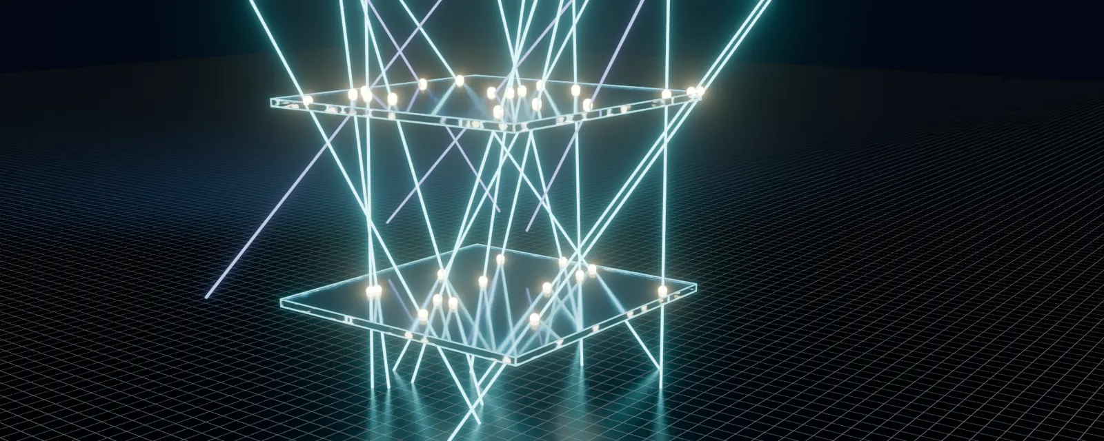
Both layers are squares of side L, separated by a distance d, with normals along the vertical. Sample N downward-going directions and N impact points on the upper layer, then count the number k of tracks that cross both layers. For this first pass use an isotropic downward hemisphere; a later step replaces it with the approximately cos²θ sea-level muon angular distribution. Keeping the beam model separate from the detector geometry is deliberate.
两层都是边长为 L 的正方形,间距为 d,法线沿竖直方向。抽样 N 个向下的方向和上层上的 N 个入射点,统计同时穿过两层的径迹数 k。第一版使用向下半球内的各向同性分布;后面一步换成近似 cos²θ 的海平面缪子角分布。把束流模型beam model与探测器几何分开,是有意为之。
The measured quantity is a conditional transmission probability: the fraction of trajectories that have already crossed the upper layer and then also cross the lower layer. It is not the full geometric acceptance of a detector exposed to a flux. The estimate and its uncertainty are
所测的量是条件透射概率:在已经穿过上层的径迹中,同时也穿过下层的比例。它不是探测器在通量照射下的完整几何接受度。估计值及其不确定度为
The count k follows a binomial distribution二项分布 Bin(N, ε) with variance Nε(1 − ε); dividing by N² gives Eq. (1.1). Raising N by a factor of 100 shrinks σε by only a factor of 10. Every later Geant4 measurement in this course pays this statistical tax.
计数 k 服从二项分布binomial distribution Bin(N, ε),方差为 Nε(1 − ε);除以 N² 即得式 (1.1)。N 增加 100 倍,σε 只缩小 10 倍——这是本课程之后每一个 Geant4 测量都要缴纳的“统计税”。
Three numbers that are easy to confuse三个容易混淆的量
| Quantity物理量 | What it is含义 | Where出现 |
|---|---|---|
| ε | Conditional transmission: of the tracks that cross the upper layer, the fraction that also cross the lower layer. Dimensionless.条件透射概率:穿过上层的径迹中,同时穿过下层的比例。无量纲。 | this week本周 |
| AΩ | Geometric acceptance几何接受度: the integral over positions and directions that turns an intensity into a rate. Units m²·sr. Needs a defined flux.几何接受度geometric acceptance:对位置和方向的积分,把强度换算成计数率。单位 m²·sr,需要先定义通量。 | wk 12 projects第 12 周项目 |
| η | Detector efficiency探测效率: of the particles that cross the detector, the fraction that produce a recorded signal above threshold.探测效率detector efficiency:穿过探测器的粒子中,产生超过阈值并被记录的信号的比例。 | week 5第 5 周 |
Think about it想一想
Before you run anything, predict: if N goes from 1,000 to 100,000, roughly how much does the relative uncertainty on the transmission probability shrink? The same 1/√N rule returns in the energy-loss scan (Week 4's lab) and the validation benchmark (Week 11's lab).
运行之前先预测:N 从 1,000 增加到 100,000,透射概率的相对不确定度大约缩小多少?同样的 1/√N 规律会在能损扫描(第 4 周的实验)和验证基准(第 11 周的实验)中再次出现。
Reading阅读3 min3 分钟
/random/setSeeds 0 01.3 · the implementation1.3 · 完整实现
Three pieces of code matter. The rest is bookkeeping.真正要紧的代码只有三处,其余都是簿记。
The full script in the hands-on task is short enough to read top to bottom in a few minutes. Before you read it, find these three pieces. If the beam model changes and the geometry does not, only the first piece should change.
动手任务里的完整脚本几分钟就能从头读到尾。读之前,先找到下面三处。如果束流模型变了而几何不变,只有第一处应该改动。
# 1. beam model: sample_directions() — cos(theta) uniform = isotropic
cos_theta = rng.uniform(0.0, 1.0, N)

# 2. geometry: straight-line propagation to the lower layer
x1 = x0 + d * np.tan(theta) * np.cos(phi)
y1 = y0 + d * np.tan(theta) * np.sin(phi)

# 3. observable: did the track land on the lower square?
hit = (np.abs(x1) < L / 2) & (np.abs(y1) < L / 2)
Intuition直觉
A Monte Carlo simulation is an opinion poll. You cannot ask every voter, which here means enumerating every possible history. If you draw enough unbiased random samples, the sample fraction converges to the true fraction at a predictable rate, and that rate is the 1/√N law. From day one, this is the ruler for a simulation's credibility.
蒙特卡罗模拟就像民意调查:你不可能问遍每一位选民(即枚举每一种可能的物理历史),但只要抽取足够多无偏的随机样本,样本比例就会以可预期的速度收敛到真实比例,这个速度就是 1/√N 规律。从第一天起,它就是衡量模拟可信度的标尺。
Interactive交互10 min10 分钟
/run/beamOn 1000interactive toy model交互玩具模型
Fire the telescope, then watch the error bar shrink as 1/√N.发射径迹,看误差棒按 1/√N 缩小。
Each button adds events to one growing sample. Change the beam model, L or d to start a new sample. The lower panels repeat the whole experiment 400 times so you can see the spread that σε predicts.
每个按钮都往同一个样本里追加事例;改变束流模型、L 或 d 会开始一个新样本。下方的面板把整个实验重复 400 次,让你看到 σε 所预言的涨落。
this sample当前样本
Reference: numerical integral of the same beam model and geometry (900 × 240 midpoints), independent of the random numbers.参考值:对同一束流模型与几何的数值积分(900 × 240 个中点),与随机数无关。
relative uncertainty vs N相对不确定度随 N 的变化
One point per click. Each tenfold step in N moves the point down by √10 ≈ 3.16.每点击一次增加一个点。N 每增大 10 倍,点下移 √10 ≈ 3.16 倍。
400 pseudo-experiments400 次伪实验
A pseudo-experiment is one complete repeat of the run with fresh random numbers. The spread of their results is what σε claims to predict.伪实验是用新的随机数把整个运行完整重复一次。它们结果的离散程度,正是 σε 声称要预言的东西。
TOY MODEL · approximations近似
Straight lines in vacuum: no energy loss, scattering or decay. Both layers are zero-thickness squares that detect every crossing. Impact points are uniform on the upper layer. Directions come from the selected beam model. The reference value integrates the same model, so agreement checks the sampling and the statistics, not the physics of real muons. The cos²θ shape is the PDG approximation for sea-level muons of a few GeV; it ignores the energy dependence of the angular distribution. Charges are drawn with μ⁺/μ⁻ ≈ 1.27 only for colour.
真空中的直线:没有能量损失、散射或衰变。两层都是零厚度的正方形,对每次穿越都 100% 响应。入射点在上层均匀分布,方向来自所选的束流模型。参考值对同一模型积分,因此两者一致只检验抽样和统计,并不检验真实缪子的物理。cos²θ 形状是 PDG 对几 GeV 海平面缪子的近似,忽略了角分布对能量的依赖。电荷按 μ⁺/μ⁻ ≈ 1.27 抽取,仅用于着色。
Hands-on lab动手实验45 min45 分钟
/control/shell python3 telescope_transmission.pyhands-on · Lab 1动手任务 · 实验 1
Run it, validate it, break it, then give it a real sky.运行、验证、破坏,再换上真实的天空。
Download all files for this lab (zip)下载本实验的全部文件(zip)all weeks全部周次
Work in your own terminal. Every expected output below was produced with NumPy 2.5.3 and the fixed seed in the script; any NumPy with default_rng should print the same digits. Tick each step when you have matched it.
在你自己的终端里完成。下面每个预期输出都是用 NumPy 2.5.3 和脚本中的固定种子得到的;任何带 default_rng 的 NumPy 版本都应输出相同的数字。对上结果后勾选该步。
-
Set up a clean Python environment建立干净的 Python 环境
terminalANALYSISpython3 -m venv ~/g4c && source ~/g4c/bin/activate pip install numpy python3 -c "import numpy; print(numpy.__version__)"
On Windows without WSL, use PowerShell instead (if activation is blocked, run
Set-ExecutionPolicy -Scope CurrentUser RemoteSignedonce). In mainland China add-i https://pypi.tuna.tsinghua.edu.cn/simpletopip install. From Week 2 on you need Linux, macOS or WSL2: see Week 0 · Set up your computer.在没有 WSL 的 Windows 上,请改用 PowerShell(如果激活被阻止,先运行一次
Set-ExecutionPolicy -Scope CurrentUser RemoteSigned)。在中国大陆,给pip install加上-i https://pypi.tuna.tsinghua.edu.cn/simple。从第 2 周起需要 Linux、macOS 或 WSL2:见第 0 周 · 配置你的电脑。Windows PowerShellANALYSISpy -3 -m venv $HOME\g4c $HOME\g4c\Scripts\Activate.ps1 pip install numpy python -c "import numpy; print(numpy.__version__)"
-
Save and run the script保存并运行脚本
telescope_transmission.pyANALYSISimport numpy as np def sample_directions(N, rng): """Sample N directions uniformly in solid angle over the downward hemisphere. This is a toy directional model. It is not the cosine-weighted crossing distribution of an isotropic flux through a plane, and it is not a sea-level cosmic-ray muon spectrum. """ # Isotropic direction sampling over a hemisphere: cos(theta) is uniform. cos_theta = rng.uniform(0.0, 1.0, N) theta = np.arccos(cos_theta) phi = rng.uniform(0.0, 2 * np.pi, N) return theta, phi def transmission_probability(N, L, d, seed=0): """Monte Carlo estimate of a two-layer telescope's conditional transmission probability. L : side length of each square layer [m] d : vertical separation between the two layers [m] The upper-layer impact point is sampled uniformly in the square. """ rng = np.random.default_rng(seed) theta, phi = sample_directions(N, rng) # Sample the impact point uniformly across the upper square. x0 = rng.uniform(-L / 2, L / 2, N) y0 = rng.uniform(-L / 2, L / 2, N) # Straight-line propagation to the lower layer. x1 = x0 + d * np.tan(theta) * np.cos(phi) y1 = y0 + d * np.tan(theta) * np.sin(phi) hit = (np.abs(x1) < L / 2) & (np.abs(y1) < L / 2) k = hit.sum() eps = k / N sigma = np.sqrt(eps * (1 - eps) / N) return eps, sigma if __name__ == "__main__": for N in [1_000, 10_000, 100_000]: eps, sigma = transmission_probability(N, L=0.3, d=0.5) print(f"N={N:>7d} eps={eps:.4f} sigma={sigma:.4f} " f"rel.unc.={sigma/eps:.2%}")
terminalpython3 telescope_transmission.py
expected output预期输出N= 1000 eps=0.0570 sigma=0.0073 rel.unc.=12.86% N= 10000 eps=0.0485 sigma=0.0021 rel.unc.=4.43% N= 100000 eps=0.0482 sigma=0.0007 rel.unc.=1.40%
Read the last column. It falls by 2.9 and then by 3.2 for each tenfold step in N, close to √10 ≈ 3.16 and nowhere near 10. The ratios are not exactly √10 because each line uses its own estimate ε̂ in the denominator.
看最后一列:N 每增大 10 倍,它分别缩小 2.9 倍和 3.2 倍,接近 √10 ≈ 3.16,远不是 10 倍。比值不严格等于 √10,是因为每一行分母里用的是各自的估计值 ε̂。
-
Validate against an independent number与独立数值比较
For L = 0.3 m and d = 0.5 m, a numerical integral of the same isotropic model gives ε = 0.04901 (SciPy
dblquad; this page's explainer computes it the same way). Run one million events and express the difference in units of σ.对 L = 0.3 m、d = 0.5 m,同一各向同性模型的数值积分给出 ε = 0.04901(SciPy
dblquad;本页演示用同样的方法计算)。运行一百万个事例,并以 σ 为单位给出差异。terminalANALYSISpython3 -c "from telescope_transmission import transmission_probability as t; e, s = t(1_000_000, L=0.3, d=0.5); print(f'eps = {e:.5f} +/- {s:.5f} pull vs 0.04901: {(e-0.04901)/s:+.2f} sigma')"expected output预期输出eps = 0.04920 +/- 0.00022 pull vs 0.04901: +0.88 sigma
A pull of +0.88σ means agreement. This compares the Monte Carlo with the model it samples. It says nothing yet about real muons.
+0.88σ 的偏差说明两者一致。这只是把蒙特卡罗与它所抽样的模型相比,还不能说明真实缪子的情况。
-
Break it on purpose: sample θ uniformly故意破坏:让 θ 均匀分布
In
sample_directions(), replace the two highlighted lines with the one below and rerun. This is a deliberately biased sampling: try it before you touch Geant4, so you see how much a wrong angular model moves the answer.在
sample_directions()中,把高亮的两行换成下面这一行,然后重新运行。这是一种故意有偏的抽样:在接触 Geant4 之前先试一试,看看错误的角分布模型会让答案偏多少。sample_directions()ANALYSIStheta = rng.uniform(0.0, np.pi / 2, N) # BROKEN: uniform in thetaexpected output预期输出N= 1000 eps=0.1500 sigma=0.0113 rel.unc.=7.53% N= 10000 eps=0.1660 sigma=0.0037 rel.unc.=2.24% N= 100000 eps=0.1699 sigma=0.0012 rel.unc.=0.70%
ε jumps from 0.049 to 0.170, with small error bars. Uniform θ ignores the sinθ in dΩ = sinθ dθ dφ and over-weights near-vertical tracks. Note the trap: 0.170 is almost exactly the value of a different, physical model (step 5). A wrong sampler can land on a plausible number, which is why you check against the model you meant.
ε 从 0.049 跳到 0.170,误差棒还很小。θ 均匀忽略了 dΩ = sinθ dθ dφ 中的 sinθ,使接近竖直的径迹权重过大。注意这个陷阱:0.170 几乎正好等于另一个合理物理模型的值(第 5 步)。错误的抽样也可能给出看似合理的数,所以必须与你本来想用的模型比较。
-
Give it a real sky: the cos²θ sea-level shape换上真实天空:海平面 cos²θ 分布
Restore the original lines. At sea level the muon intensity per solid angle is approximately I(θ) ∝ cos²θ (PDG, Cosmic rays review, for muons of a few GeV). The density of c = cosθ is then 3c² on [0, 1], its cumulative distribution is c³, and inverting it gives c = u1/3 for uniform u. Only the beam model changes.
先恢复原来的两行。海平面上缪子的单位立体角强度近似为 I(θ) ∝ cos²θ(PDG 宇宙线综述,适用于几 GeV 的缪子)。于是 c = cosθ 在 [0, 1] 上的概率密度为 3c²,累积分布为 c³,反解得 c = u1/3(u 均匀)。只改动束流模型。
sample_directions()ANALYSIScos_theta = rng.uniform(0.0, 1.0, N) ** (1 / 3) # pdf of cos(theta) ~ cos^2 theta = np.arccos(cos_theta)expected output预期输出N= 1000 eps=0.1490 sigma=0.0113 rel.unc.=7.56% N= 10000 eps=0.1340 sigma=0.0034 rel.unc.=2.54% N= 100000 eps=0.1341 sigma=0.0011 rel.unc.=0.80%
Reference integral: 0.1336. Muons crossing a horizontal layer carry one more factor of cosθ (the projected area), so the crossing distribution goes as cos³θ and c = u1/4. Try it: you should get 0.1699 at N = 100,000 against a reference of 0.1702. The script's first-pass model, isotropic per solid angle, is neither of these, as its docstring warns.
参考积分值为 0.1336。穿过水平探测层的缪子还要再乘一个 cosθ(投影面积),所以穿越分布为 cos³θ,c = u1/4。试一试:N = 100,000 时应得到 0.1699,参考值为 0.1702。脚本中第一版的“单位立体角各向同性”模型两者都不是,正如它的文档字符串所提醒的。
-
Fill in the research notebook填写研究笔记
Write these five lines for Lab 1 before you start Week 2. If you can complete them, you already think like a simulation experimentalist.
在开始第 2 周之前,为实验 1 写下这五行。如果你能写完,你已经在像模拟实验者一样思考了。
Question What physical quantity am I trying to learn?问题:我想知道哪个物理量? Prediction What should happen, and why?预测:应该发生什么?为什么? Observable What number will the simulation actually produce?可观测量:模拟实际会输出哪个数? Validation What independent expectation or data will I compare with?验证:我将与哪个独立预期或数据比较? Limitation What important part of reality is still missing?局限:还缺少现实中的哪个重要部分? -
Prepare for Week 2: install and check Geant4为第 2 周做准备:安装并检查 Geant4
Next week the same experiment moves into Geant4. The core weeks target Geant4 11.4 with C++17. If you have not installed it yet, follow Week 0 · Set up your computer now (plan 1–3 hours; Windows users go through WSL2 or the container). Then activate your Geant4 environment and run:
下周同一个实验将搬进 Geant4。核心周次以 Geant4 11.4 和 C++17 为目标。如果还没有安装,现在就按第 0 周 · 配置你的电脑操作(预留 1–3 小时;Windows 用户通过 WSL2 或容器)。然后激活 Geant4 环境并运行:
terminalGEANT4geant4-config --version geant4-config --check-datasets cmake --version
expected预期11.4.x # any 11.4 patch release # --check-datasets: every data library reported as installed, none missing cmake version 3.16 or newer
There is no generic
geant4 --versioncommand. Ifgeant4-configis not found, your Geant4 environment has not been activated (conda activate g4c, orsource <install>/bin/geant4.sh). ROOT is not needed now: Weeks 2–8 and 11–12 read output with Python (uproot). ROOT is only needed for musrSim in Weeks 9–10, and the setup page covers it.并不存在通用的
geant4 --version命令。如果找不到geant4-config,说明还没有激活 Geant4 环境(conda activate g4c,或source <安装目录>/bin/geant4.sh)。现在不需要 ROOT:第 2–8 周和第 11–12 周都用 Python(uproot)读取输出。只有第 9–10 周的 musrSim 需要 ROOT,配置页面里有说明。
Practice quiz练习测验9 min9 分钟
/control/verbose 2self-check自测
Six questions. Each answer explains itself.六道题,每个答案都附有解释。
Reading阅读12 min12 分钟
G4Exceptioncommon errors常见错误
Six mistakes that run without a single error message.六个不会报任何错的错误。
Checklist清单5 min5 分钟
/control/saveHistoryreview notes复习要点
Before you close the run.结束运行之前。
Remark · debt repaid, debt taken on小结 · 还清的债与新欠的债
Repaid: random sampling, conditional transmission probability and statistical uncertainty are now numbers you computed yourself. Taken on: all of it happened in a matter-free toy world where particles fly in straight lines and lose no energy. Next week the particle enters the Geant4 world, and Week 4's lab will ask how much it loses when it crosses matter.
还清的债:随机抽样、条件透射概率和统计不确定度,已经是你亲手算出的数字。新欠的债:这一切都发生在没有物质、没有能损、粒子走直线的“真空玩具世界”里。下周粒子将进入 Geant4 的世界,而第 4 周的实验会追问:粒子穿过物质时究竟损失多少能量?
Share分享5 min5 分钟
/vis/ogl/export week01.gifshare this week分享本周成果
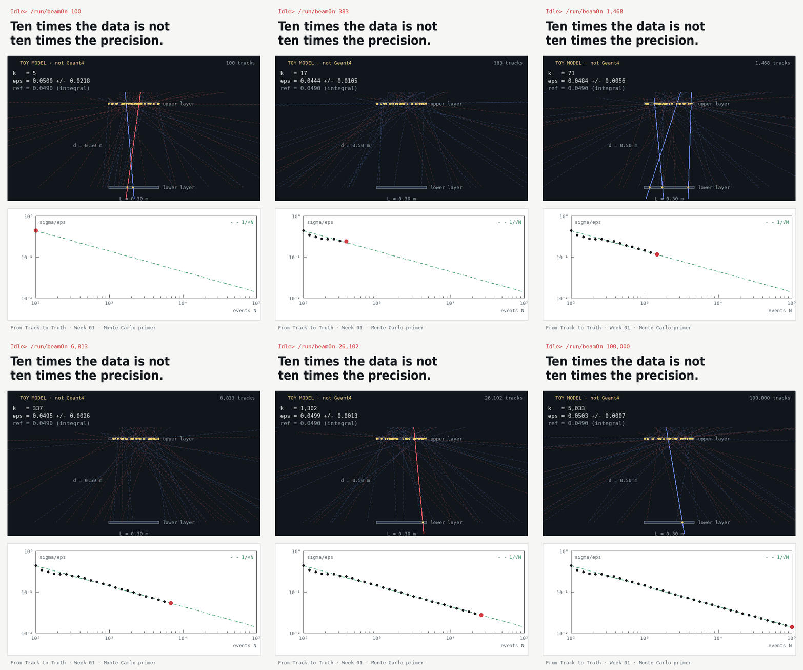
Ten times the data is not ten times the precision.十倍的数据,不等于十倍的精度。
Post your three-line output with the GIF and one sentence on what surprised you. Then rerun step 3 with seed= your student number and share the pull in the course group. Across the class, about two thirds of the pulls should fall within ±1σ, and about one in twenty outside ±2σ.
把你的三行输出、这张 GIF 和一句“最让我意外的是……”发出来。然后用 seed=你的学号重新运行第 3 步,把偏差发到课程群里。全班的偏差中,大约三分之二应落在 ±1σ 以内,约二十分之一落在 ±2σ 之外。